genesis-oracle
Genesis Oracle
Week 2 – Keras + RC Filter
- Keras 3 with JAX backend ✔
- Fourier square wave generation ✔
- RC low-pass filtering ✔
- Noise + anomaly injection ✔
See:
- data_feed.png
- src/data_generator.py
Agent Simulation Report
Execution Summary
The simulation script src/ancients.py has been successfully executed.
The process ran without errors using the provided virtual environment (nexus_env), and the output plot was successfully generated and saved to the designated directory as data/ancients_plot.png.
Simulated Systems
The script simulates two distinct physical systems:
- Harmonic Oscillator: Simulated using a system of two first-order differential equations (position and velocity) with an angular frequency $\omega = 2.0$.
- Radioactive Decay: Simulated using a first-order differential equation modeling exponential decay over time, with a decay constant $\alpha = 0.5$.
Both systems were integrated over a time interval of $t \in [0, 10]$ using SciPy’s solve_ivp with the Runge-Kutta 4(5) method. The visual results were successfully plotted side-by-side in the output file.
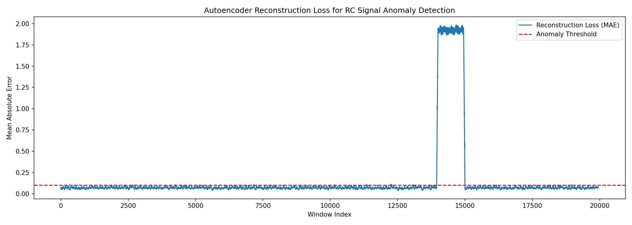
Week 3: Oracle Awakens — Autoencoder Anomaly Detection
In this experiment, I trained a subclassed Keras 3 autoencoder on the normal part of a synthetic RC-filter signal. The model learned to reconstruct normal signal windows with low error. When the corrupted anomaly region was passed through the model, the reconstruction error increased strongly, creating a clear spike above the anomaly threshold.
Conv1D Refactoring
The dense autoencoder was extended with a Conv1D-based architecture. Conv1D layers are better suited for time-series signals because they apply local filters across neighboring time steps. This helps the model capture local structures such as oscillations, short distortions, and voltage spikes while preserving temporal order.